Example: efficiently training a Seldonian facial recognition system
We will now go through an example to make the steps described in the outline above more concrete. We will use the same dataset and model from the Gender bias in facial recognition example. In that example, we trained a convolutional neural network (CNN) to classify gender from images of faces from the UTKFace dataset, subject to a fairness constraint enforcing that accuracy should be similar when predicting male and female faces. Before following along with the steps above, we need to set up our computing environment properly. We recommend following along with these steps in the Colab notebook linked at the top of this tutorial. However, we reproduce the steps here if you simply want to read along rather than run the cells yourself.
Preliminaries
Make sure GPU is enabled
Make sure that whatever system you're on is capable of using the GPU. The Colab notebook (link at the top of this page) shows how to do that for Colabs, but in general this amounts to downloading the correct drivers for PyTorch or Tensorflow.
Imports
import os
import numpy as np
import pandas as pd
from torch.utils.data import DataLoader
import torch
import torch.nn as nn
from torch import optim
from torch.autograd import Variable
from sklearn.metrics import log_loss,accuracy_score

from seldonian.spec import SupervisedSpec
from seldonian.dataset import SupervisedDataSet
from seldonian.models import objectives
from seldonian.seldonian_algorithm import SeldonianAlgorithm
from seldonian.parse_tree.parse_tree import (
    make_parse_trees_from_constraints)
from seldonian.utils.io_utils import load_pickle,save_pickle
from seldonian.utils.plot_utils import plot_gradient_descent
from experiments.generate_plots import SupervisedPlotGenerator
Dataset preparation
First download the dataset from here. Unzip that file, revealing the data file called age_gender.csv. The following code loads the dataset, shuffles it, and clip off 5 samples to make the dataset size more easily divisible when making mini-batches.
torch.manual_seed(0)
regime='supervised_learning'
sub_regime='classification'

N=23700

savename_features = './features.pkl'
savename_labels = './labels.pkl'
savename_sensitive_attrs = './sensitive_attrs.pkl'

print("loading data...")
data = pd.read_csv('age_gender.csv')
print("done")
print("resampling data and clipping off 5 samples..")
data_resamp = data.sample(n=len(data),random_state=42).iloc[:N]
print("done")
The next steps are to make the features and labels that we will use to train the model. This requires converting the flattened image data from the dataframe into the shape and data type that the model expects. After creating these, we save them to disk for fast loading later.
print("Converting pixels to array...")
data_resamp['pixels']=data_resamp['pixels'].apply(lambda x:  np.array(x.split(), dtype="float32"))
print("done")

print("Normalizing and reshaping pixel data...")
data_resamp['pixels'] = data_resamp['pixels'].apply(lambda x: x/255)
print("done")

X = np.array(data_resamp['pixels'].tolist())

features = X.reshape(X.shape[0],1,48,48) # the shape expected in the model

labels = data_resamp['gender'].values

save_pickle(savename_features,features)
save_pickle(savename_labels,labels)
Step 1. Split data into two datasets
We'll call these the candidate ("cand") and safety, and use a 50/50 split. The data are already shuffled, so we'll split right down the middle. The first half will be candidate data and the second will be safety. We'll also make the PyTorch data loaders which come in handy for training with PyTorch.
# N/2 = 11850
features_cand = features[:11850]
features_safety = features[11850:]
labels_cand = labels[:11850]
labels_safety = labels[11850:]

# Convert to tensors for training with Pytorch
features_cand_tensor = torch.from_numpy(features_cand)
features_safety_tensor = torch.from_numpy(features_safety)
labels_cand_tensor = torch.from_numpy(labels_cand)
labels_safety_tensor = torch.from_numpy(labels_safety)

# Make torch data loaders
batch_size = 100
candidate_dataset=torch.utils.data.TensorDataset(
    features_cand_tensor,labels_cand_tensor)
candidate_dataloader=torch.utils.data.DataLoader(
    candidate_dataset,batch_size=batch_size,shuffle=False)
safety_dataset=torch.utils.data.TensorDataset(
    features_safety_tensor,labels_safety_tensor)
safety_dataloader=torch.utils.data.DataLoader(
    safety_dataset,batch_size=batch_size,shuffle=False)
loaders = {
    'candidate' : candidate_dataloader,
    'safety'  : safety_dataloader
}
Step 2. Train the full network on the candidate data only
Let's define the full network below.
class CNNModelNoSoftmax(nn.Module):
    def __init__(self):
        # Model used for training in Pytorch only. No droputs, no softmax
        super(CNNModelNoSoftmax, self).__init__()

        self.cnn1 = nn.Conv2d(in_channels=1, out_channels=16, kernel_size=3, padding=1)
        self.relu = nn.ReLU()

        # Max pool 1
        self.maxpool = nn.MaxPool2d(kernel_size=2)

        self.Batch1=nn.BatchNorm2d(16)
        self.Batch2=nn.BatchNorm2d(32)
        self.Batch3=nn.BatchNorm2d(64)
        self.Batch4=nn.BatchNorm2d(128)


        self.cnn2 = nn.Conv2d(in_channels=16, out_channels=32, kernel_size=3)
        self.cnn3 = nn.Conv2d(in_channels=32, out_channels=64, kernel_size=3)
        self.cnn4 = nn.Conv2d(in_channels=64, out_channels=128, kernel_size=3)

        # Fully connected 1 (readout)
        self.fc1 = nn.Linear(128 * 1 * 1, 128)
        self.fc2=nn.Linear(128,256)
        self.fc3=nn.Linear(256,2)

    def forward(self, x):

        out = self.cnn1(x)
        out = self.relu(out)
        out = self.maxpool(out)
        out = self.Batch1(out)

        out = self.cnn2(out)
        out = self.relu(out)
        out = self.maxpool(out)
        out = self.Batch2(out)

        out = self.cnn3(out)
        out = self.relu(out)
        out = self.maxpool(out)
        out = self.Batch3(out)

        out = self.cnn4(out)
        out = self.relu(out)
        out = self.maxpool(out)
        out = self.Batch4(out)


        # Resize
        # Original size: (100, 32, 7, 7)
        # out.size(0): 100
        # New out size: (100, 32*7*7)
        out = out.view(out.size(0), -1)
        # Linear function (readout)
        out = self.fc1(out)
        out = self.fc2(out)
        out = self.fc3(out)

        return out
Next, we instantiate the model, and put it on the GPU.
cnn = CNNModelNoSoftmax()
cnn.to(device) # puts it on the GPU
Here, we set up the training parameters and the training function.
learning_rate=0.001
loss_func = nn.CrossEntropyLoss()
optimizer = torch.optim.Adam(cnn.parameters(), lr=learning_rate)

def train(num_epochs, cnn, loaders):

    cnn.train()

    # Train the model
    total_step = len(loaders['candidate'])

    for epoch in range(num_epochs):
        for i, (images, labels) in enumerate(loaders['candidate']):

            images = images.to(device)
            labels = labels.to(device)
            b_x = Variable(images)   # batch x
            output = cnn(b_x)
            b_y = Variable(labels)   # batch y
            loss = loss_func(output, b_y)

            # clear gradients for this training step
            optimizer.zero_grad()

            # backpropagation, compute gradients
            loss.backward()
            # apply gradients
            optimizer.step()

            if (i+1) % 100 == 0:
                print ('Epoch [{}/{}], Step [{}/{}], Loss: {:.4f}'
                       .format(epoch + 1, num_epochs, i + 1, total_step, loss.item()))
Let's train for ten epochs.
num_epochs = 10
train(num_epochs, cnn, loaders)
Running that code produces the following output:
Training model on full CNN with 10 epochs
Epoch [1/10], Step [100/119], Loss: 0.3644
Epoch [2/10], Step [100/119], Loss: 0.2790
Epoch [3/10], Step [100/119], Loss: 0.2157
Epoch [4/10], Step [100/119], Loss: 0.1937
Epoch [5/10], Step [100/119], Loss: 0.2020
Epoch [6/10], Step [100/119], Loss: 0.2036
Epoch [7/10], Step [100/119], Loss: 0.1336
Epoch [8/10], Step [100/119], Loss: 0.0666
Epoch [9/10], Step [100/119], Loss: 0.0720
Epoch [10/10], Step [100/119], Loss: 0.0973
done.
We evaluate the performance on the safety dataset using the following code.
def test():
    cnn.eval()
    test_loss = 0
    correct = 0
    test_loader = loaders['safety']
    with torch.no_grad():
        for images, target in test_loader:
            images = images.to(device)
            target = target.to(device)
            output = cnn(images)
            pred = output.data.max(1, keepdim=True)[1]
            correct += pred.eq(target.data.view_as(pred)).sum()
    print('\nTest set: Accuracy: {}/{} ({:.0f}%)\n'.format(
    correct, len(test_loader.dataset),
    100. * correct / len(test_loader.dataset)))
test()
Running that code produces the following output:
Test set: Accuracy: 10195/11850 (86%)
The result may differ slightly depending on your machine and random seed. We need to save the parameters of this trained model so we can apply them to the body-only model.
# Save state dict after training and verify parameters were changed
sd_after_training = cnn.state_dict()
Step 3. Separate out the "body" and the "head" of the full network into two separate models
The body-only model is the full network minus the final fully connected layer (and the softmax):
# Defines the body-only a.k.a "headless" model
class CNNHeadlessModel(nn.Module):
    # Model for creating latent features. No dropouts, no final fc3 layer and no softmax
    def __init__(self):
        super(CNNHeadlessModel, self).__init__()

        self.cnn1 = nn.Conv2d(in_channels=1, out_channels=16, kernel_size=3, padding=1)
        self.relu = nn.ReLU()

        # Max pool 1
        self.maxpool = nn.MaxPool2d(kernel_size=2)

        self.Batch1=nn.BatchNorm2d(16)
        self.Batch2=nn.BatchNorm2d(32)
        self.Batch3=nn.BatchNorm2d(64)
        self.Batch4=nn.BatchNorm2d(128)

        self.cnn2 = nn.Conv2d(in_channels=16, out_channels=32, kernel_size=3)
        self.cnn3 = nn.Conv2d(in_channels=32, out_channels=64, kernel_size=3)
        self.cnn4 = nn.Conv2d(in_channels=64, out_channels=128, kernel_size=3)

        # Fully connected 1 (readout)
        self.fc1 = nn.Linear(128 * 1 * 1, 128)
        self.fc2=nn.Linear(128,256)

    def forward(self, x):

        out = self.cnn1(x)
        out = self.relu(out)
        out = self.maxpool(out)
        out=self.Batch1(out)

        out = self.cnn2(out)
        out = self.relu(out)
        out = self.maxpool(out)
        out=self.Batch2(out)

        out = self.cnn3(out)
        out = self.relu(out)
        out = self.maxpool(out)
        out=self.Batch3(out)

        out = self.cnn4(out)
        out = self.relu(out)
        out = self.maxpool(out)
        out=self.Batch4(out)

        # Resize
        # Original size: (100, 32, 7, 7)
        # out.size(0): 100
        # New out size: (100, 32*7*7)
        out = out.view(out.size(0), -1)

        # Linear function (readout)
        out = self.fc1(out)

        out=self.fc2(out)

        return out
Let's instantiate this model and put it on the GPU.
cnn_headless = CNNHeadlessModel().to(device)
Step 4. Assign the weights from the trained full network to the new body-only model
This ensures that the body-only model is "trained." Remove the weights and bias from the last layer of the state dictionary from the trained full model so that we can copy the state dict from the trained model to the new headless model.
del sd_after_training['fc3.weight']
del sd_after_training['fc3.bias']

cnn_headless.load_state_dict(sd_after_training)
Step 5. Pass all of the data (both datasets from step 1) through the trained "body-only" model
Save the outputs of passing the data through the model. These are your new "latent features" that you will use as input to the Seldonian Toolkit. First, notice that the output of the last layer of the headless model has size: 256. Therefore, we will have 256 features for each image.
Pass candidate data in first, followed by safety data. When we use these features/labels in the Seldonian Toolkit, the candidate data are taken first during the candidate/safety split. This code also fills the labels we will save. The last part of the code saves the features and labels to pickle files.
new_features = np.zeros((23700,256))
new_labels = np.zeros(23700)
batch_size=100
for i,(images, labels) in enumerate(loaders['candidate']):
    images = images.to(device)
    start_index = i*batch_size
    end_index = start_index + len(images)
    new_labels[start_index:end_index] = labels.numpy()
    new_features[start_index:end_index] = cnn_headless(images).cpu().detach().numpy()
for j,(images, labels) in enumerate(loaders['safety']):
    images = images.to(device)
    start_index = end_index
    end_index = start_index + len(images)
    new_labels[start_index:end_index] = labels.numpy()
    new_features[start_index:end_index] = cnn_headless(images).cpu().detach().numpy()

# Save latent features and labels
save_pickle('facial_gender_latent_features.pkl',new_features)
save_pickle('facial_gender_labels.pkl',new_labels)
Step 6. The head-only model is the model we will use in the toolkit
The head-only model should be initially untrained when used in the toolkit, so don't apply the weights learned in step 2 to the head. The model needs to be compatible with the toolkit, so regardless of the programming language used to define the full network, the head-only model needs to be implemented in Python. Specifically, the toolkit supports Numpy, PyTorch or Tensorflow models. We will just take the PyTorch implemented of the head from the full network and implement it as its own model.
from seldonian.models.pytorch_model import SupervisedPytorchBaseModel

class FacialRecogHeadCNNModel(nn.Module):
    def __init__(self):
        """ Implements just the linear + softmax output layer
        of the full CNN
        """
        super(FacialRecogHeadCNNModel, self).__init__()

        self.fc3=nn.Linear(256,2)
        self.softmax = nn.Softmax(dim=1)

    def forward(self, x):

        out=self.fc3(x)
        out=self.softmax(out)[:,1]

        return out

class PytorchFacialRecogHead(SupervisedPytorchBaseModel):
    def __init__(self,device):
        """
        The Seldonian model, implementing just the head of the
        full CNN.
        """
        super().__init__(device)

    def create_model(self,**kwargs):
        return FacialRecogHeadCNNModel()
Step 7. The data we will use are the latent features created in step 5
Let's create a Seldonian dataset object from these features, the labels and the sensitive attributes
print("Making SupervisedDataSet...")

savename_features = './facial_gender_latent_features.pkl'
savename_labels = './facial_gender_labels.pkl'
features = load_pickle(savename_features)
labels = load_pickle(savename_labels)
F = load_pickle(savename_labels) # the labels are 0 if male 1 if female
mask=~(F.astype("bool"))
M=mask.astype('int64')
sensitive_attrs = np.hstack((M.reshape(-1,1),F.reshape(-1,1)))

sensitive_col_names = ['M','F']

meta_information = {}
meta_information['feature_col_names'] = ['img']
meta_information['label_col_names'] = ['label']
meta_information['sensitive_col_names'] = sensitive_col_names
meta_information['sub_regime'] = sub_regime

dataset = SupervisedDataSet(
  features=features,
  labels=labels,
  sensitive_attrs=sensitive_attrs,
  num_datapoints=N,
  meta_information=meta_information)
print("done")
Step 8. Assign the frac_data_in_safety parameter of the spec object to be the same split fraction as you used in step 1
We used a 50/50 split in step 1, so we just need to set frac_data_in_safety=0.5. Recall that the candidate data that we use in the toolkit must match the dataset that we used to train the full model in step 2. In other words, no safety data should come from the dataset that was used to train the full model in step 2 because that would invalidate the safety/fairness guarantees. The data split that the toolkit performs does not reshuffle the data, so the candidate data will be the first half of the data we pass to the dataset object. This is the same half on which we trained the full model. That means that the latent features that will be used as candidate data in the toolkit came from the candidate data on which we trained the full model.
Step 9. Run the Seldonian Engine/Experiments as normal, except now the model is a simple linear model instead of a deep network
As we will see, using the head-only in the toolkit will be much faster than using the full network as we did in the Gender bias in facial recognition example. Let's set up the spec object we need to run the Engine. We already have the dataset object, so we just need the parse trees and the hyperparameters for the optimization. Note that we don't need to use mini-batches in gradient descent/ascent because the model is now a small linear model and no longer a deep network.
constraint_strs = ['min((ACC | [M])/(ACC | [F]),(ACC | [F])/(ACC | [M])) >= 0.8']
deltas = [0.05]
print("Making parse trees for constraint(s):")
print(constraint_strs," with deltas: ", deltas)
parse_trees = make_parse_trees_from_constraints(
  constraint_strs,deltas,regime=regime,
  sub_regime=sub_regime,columns=sensitive_col_names)
print("done")

# Set the model to be the head-only model
# Let's run on the CPU because it's just a linear model - no need for GPU.
cpu_device = torch.device("cpu")
model = PytorchFacialRecogHead(cpu_device)

# Set the rest of the spec parameters.
# All of these are the same as what we used in the
# gender classifier example.
initial_solution_fn = model.get_model_params
primary_objective_fn = objectives.binary_logistic_loss

# Make the spec object and save it
spec = SupervisedSpec(
        dataset=dataset,
        model=model,
        parse_trees=parse_trees,
        frac_data_in_safety=frac_data_in_safety,
        primary_objective=primary_objective_fn,
        use_builtin_primary_gradient_fn=False,
        sub_regime=sub_regime,
        initial_solution_fn=initial_solution_fn,
        optimization_technique='gradient_descent',
        optimizer='adam',
        optimization_hyperparams={
            'lambda_init'   : np.array([0.5]),
            'alpha_theta'   : 0.01,
            'alpha_lamb'    : 0.01,
            'beta_velocity' : 0.9,
            'beta_rmsprop'  : 0.95,
            'use_batches'   : False,
            'num_iters'     : 1200,
            'gradient_library': "autograd",
            'hyper_search'  : None,
            'verbose'       : True,
        }
    )
save_pickle('./spec.pkl',spec,verbose=True)
Now we are ready to run the Seldonian Engine.
# Run the Seldonian Engine
SA = SeldonianAlgorithm(spec)
passed_safety,solution = SA.run(debug=False,write_cs_logfile=True)
If we run the above code, we can see that it passed the safety test, and it took less than 10 seconds on the CPU. Let's visualize the gradient descent process. Unless you are running this in Google Colab, you will probably need to change the path to the log file.
f='/content/logs/candidate_selection_log0.p'
sol_dict = load_pickle(f)
fig=plot_gradient_descent(sol_dict,primary_objective_name='cross entropy',plot_running_avg=True)
Running this code produces the following plot:
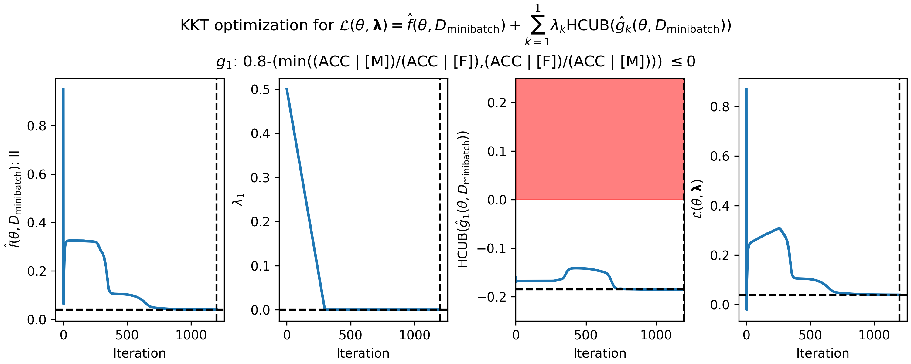 Figure 1 - How the parameters of the KKT optimization problem changed during gradient descent on the fair gender classifier example, using the linear head-only model. (Left) cross-entropy value in each mini-batch, (middle left) single Lagrange multiplier (middle right) predicted high-confidence upper bound (HCUB) on the disparate impact constraint function, $\hat{g}_1(\theta,D_\mathrm{minibatch})$, and (right) the Lagrangian $\mathcal{L}(\theta,\boldsymbol{\lambda})$. The black dotted lines in each panel indicate where the optimum was found. The optimum is defined as the feasible solution with the lowest value of the primary objective. A feasible solution is one where $\mathrm{HCUB}(\hat{g}_i(\theta,D_\mathrm{cand})) \leq 0, i \in \{1 ... n\}$. In this example, we only have one constraint, and the infeasible region is shown in red in the middle right plot.
Run a Seldonian Experiment
Note: Running the following experiments is compute-intensive on the CPU. The experiments library is parallelized across multiple CPUs to speed up the computation. However, free-tier Colab notebooks such as the default one that opens when clicking the button at the top of this tutorial lack the number and quality of CPUs for running the experiments in a reasonable amount of time. In the Colab notebook, we prepopulated the results so that the experiments did not actually have to run. However, if you want to run these experiments yourself in full, we recommend using a machine with at least 4 CPUs. For reference, on a Mac M1 with 7 CPU cores the experiment takes between between 5 and 10 minutes to complete. Though we have not tested this code in Google Colab PRO or PRO+ notebooks, we expect that the resources allocated in those paid-tier notebooks will be sufficient to run the full experiment.
Now, we set up the parameters of the experiment. We will be using 10 trials with six data fractions. This setup is similar to the setup in the gender classifier example. Set n_workers to the number of CPUs you want to use. Each CPU will get one trial at a time. Change results_dir to where you want to save the results.
# Parameter setup
cpu_device = torch.device("cpu") # run on the CPU since we have a simple linear model
include_legend = True
performance_metric = 'Accuracy'
model_label_dict = {
  'qsa':'CNN (QSA on head only)',
  'qsa_fullmodel':'CNN (QSA on full model)',
  'facial_recog_cnn': 'full CNN (no constraints)'}

n_trials = 10
data_fracs = [0.001,0.005,0.01,0.1,0.33,0.66]
batch_epoch_dict = {
  0.001:[24,50],
  0.005:[119,50],
  0.01:[237,75],
  0.1:[237,30],
  0.33:[237,20],
  0.66:[237,10],
  1.0: [237,10]
}
n_workers = 8
results_dir = '.'
verbose=False
os.makedirs(results_dir,exist_ok=True)
Here we define the ground truth dataset, which is the original dataset.
# Use entire original dataset as ground truth for test set
dataset = spec.dataset
test_features = dataset.features
test_labels = dataset.labels
Next, we define the function used for evaluating the performance and its keyword arguments. Above, we set performance_metric='Accuracy', so that's the metric we will use for the left-most plot.
# Setup performance evaluation functions and kwargs
def perf_eval_fn(y_pred,y,**kwargs):
  if performance_metric == 'log_loss':
    return log_loss(y,y_pred)
  elif performance_metric == 'Accuracy':
    return accuracy_score(y,y_pred > 0.5)

perf_eval_kwargs = {
  'X':test_features,
  'y':test_labels,
  'device':cpu_device,
  'eval_batch_size':2000
  }
We will use the default constraint evaluation function (built-in to the Engine), so we don't need to specify anything for that, but we can batch the model forward pass when evaluating the constraints. To specify the batch size, we use the following dictionary:
# Use default constraint eval function (don't need to set anything for that)
# Define kwargs to pass the the constraint eval function
constraint_eval_kwargs = {
  'eval_batch_size':2000
  }
Now we can make the plot generator and run the Seldonian experiment:
# Make the plot generator
plot_generator = SupervisedPlotGenerator(
        spec=spec,
        n_trials=n_trials,
        data_fracs=data_fracs,
        n_workers=n_workers,
        datagen_method='resample',
        perf_eval_fn=perf_eval_fn,
        constraint_eval_fns=[],
        constraint_eval_kwargs=constraint_eval_kwargs,
        results_dir=results_dir,
        perf_eval_kwargs=perf_eval_kwargs,
        batch_epoch_dict=batch_epoch_dict,
        )

# Run Seldonian experiment
plot_generator.run_seldonian_experiment(verbose=verbose)
Running the above code will produce 10 trials for each data fraction, resulting in a total of 60 files. These will be saved as CSV files in ${results_dir}/qsa_results/trial_data, where ${results_dir} is whatever you set that variable to be. We want to compare these results to the same experiment using the full deep network with the constraint as well as the full network without the constraint - these are the two curves shown in Figure 3 of the Gender bias in facial recognition example. To do this, we can copy the results from that experiment into the results_dir folder of this experiment. We did that, but renamed the qsa_results/ folder from the other experiment to qsa_fullmodel_results/ so that it wouldn't overwrite our qsa_results/ folder. The other folder we need to copy from that experiment is the facial_recog_cnn/ folder, which contains the results for the experiment on the full network lacking the constraint.
You'll notice in the parameter setup section of the current experiment that we defined the dictionary:
model_label_dict = {
  'qsa':'CNN (QSA on head only)',
  'qsa_fullmodel':'CNN (QSA on full model)',
  'facial_recog_cnn': 'full CNN (no constraints)'}
This dictionary maps the model name (the prefix to _results in the model results folder path) to the name you want displayed in the legend of the plot. Let's now run the code to make the three plots for this experiment and the two experiments we copied over.
plot_generator.make_plots(
  model_label_dict=model_label_dict,fontsize=12,legend_fontsize=8,
  performance_label=performance_metric,
  include_legend=include_legend)
Running that code produces the following three plots.
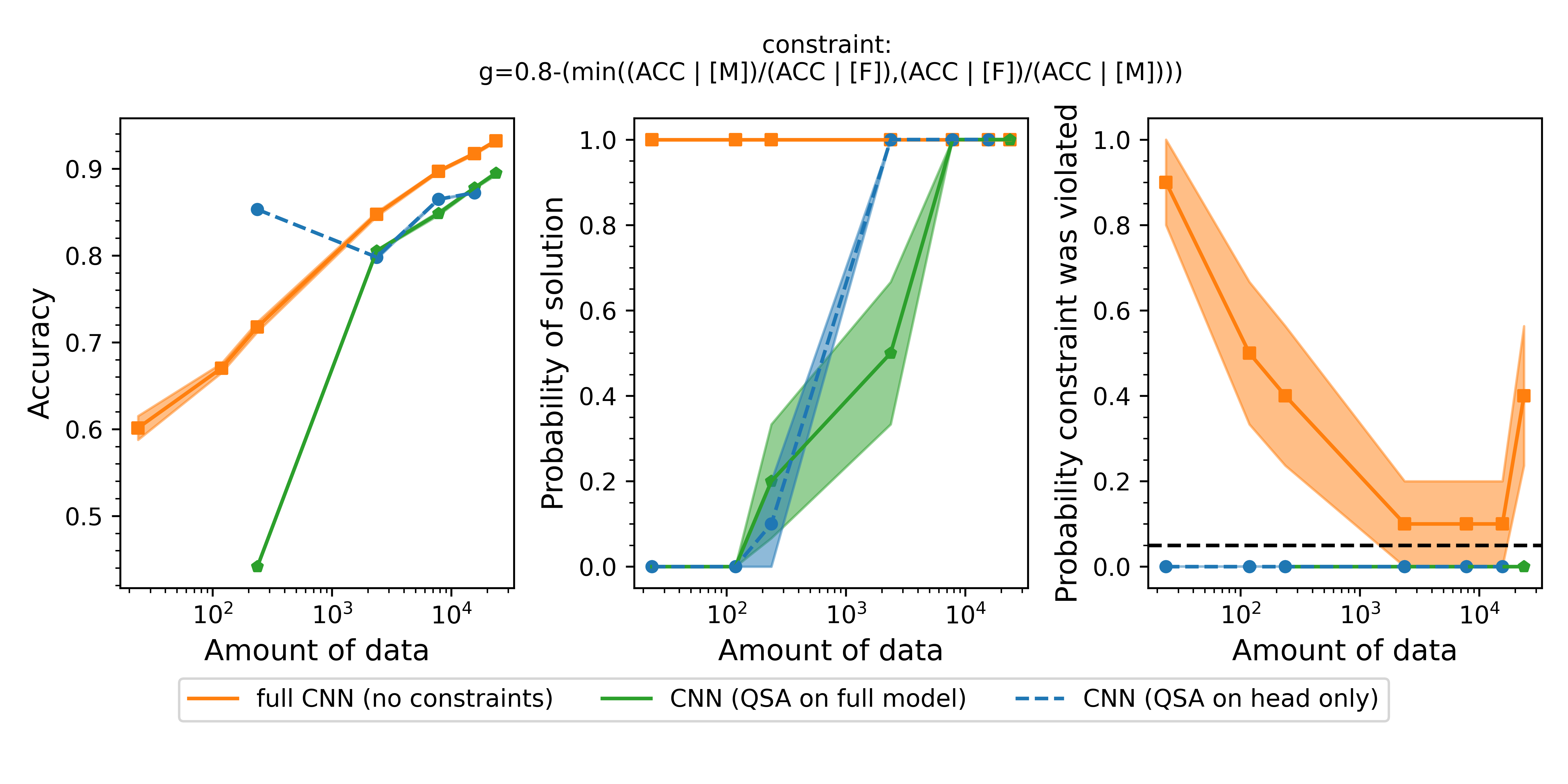 Figure 2 Accuracy (left), probability of solution (middle) and probability that the constraint was violated (right) for three different models. The orange model is the full convolutional neural network trained without any constraints. It has the highest accuracy (left), but violates the constraint frequently (right). The green model is the QSA using the full network. Running an experiment with this model is very slow because all of the parameters in all layers of the network need to be trained subject to the constraint. The blue model is the model we built in this tutorial. It has 256 parameters versus the 147,682 parameters (only 0.2%!) of the full network. Despite being a vastly simpler model, it performs as well as the full network and it similarly never violates the fairness constraint.